医学图像预处理
1)搭建运行环境,运行Brain Tumor Detection代码中裁剪功能
预先安装好相关模块,安装Jupyter Notebook交互式计算环境
conda install jupyter
首先导入相关包
import tensorflow as tf
from tensorflow.keras.layers import Conv2D, Input, ZeroPadding2D, BatchNormalization, Activation, MaxPooling2D, Flatten, Dense
from tensorflow.keras.models import Model, load_model
from tensorflow.keras.callbacks import TensorBoard, ModelCheckpoint
from sklearn.model_selection import train_test_split
from sklearn.metrics import f1_score
from sklearn.utils import shuffle
import cv2
import imutils
import numpy as np
import matplotlib.pyplot as plt
import time
from os import listdir

%matplotlib inline
因为这里只是进行图形预处理,对Brain Tumor图片进行裁剪,主要用到的包是cv2, imutils, numpy, matplotlib.pyplot
然后是运行定义裁剪脑轮廓(查找大脑的顶部、底部、左端、右端的极点)的函数(crop_brain_contour)
def crop_brain_contour(image, plot=False):

    #import imutils
    #import cv2
    #from matplotlib import pyplot as plt

    # Convert the image to grayscale, and blur it slightly
    gray = cv2.cvtColor(image, cv2.COLOR_BGR2GRAY)
    gray = cv2.GaussianBlur(gray, (5, 5), 0)

    # Threshold the image, then perform a series of erosions +
    # dilations to remove any small regions of noise
    thresh = cv2.threshold(gray, 45, 255, cv2.THRESH_BINARY)[1]
    thresh = cv2.erode(thresh, None, iterations=2)
    thresh = cv2.dilate(thresh, None, iterations=2)

    # Find contours in thresholded image, then grab the largest one
    cnts = cv2.findContours(thresh.copy(), cv2.RETR_EXTERNAL, cv2.CHAIN_APPROX_SIMPLE)
    cnts = imutils.grab_contours(cnts)
    c = max(cnts, key=cv2.contourArea)


    # Find the extreme points
    extLeft = tuple(c[c[:, :, 0].argmin()][0])
    extRight = tuple(c[c[:, :, 0].argmax()][0])
    extTop = tuple(c[c[:, :, 1].argmin()][0])
    extBot = tuple(c[c[:, :, 1].argmax()][0])

    # crop new image out of the original image using the four extreme points (left, right, top, bottom)
    new_image = image[extTop[1]:extBot[1], extLeft[0]:extRight[0]]

    if plot:
        plt.figure()

        plt.subplot(1, 2, 1)
        plt.imshow(image)

        plt.tick_params(axis='both', which='both',
                        top=False, bottom=False, left=False, right=False,
                        labelbottom=False, labeltop=False, labelleft=False, labelright=False)

        plt.title('Original Image')

        plt.subplot(1, 2, 2)
        plt.imshow(new_image)

        plt.tick_params(axis='both', which='both',
                        top=False, bottom=False, left=False, right=False,
                        labelbottom=False, labeltop=False, labelleft=False, labelright=False)

        plt.title('Cropped Image')

        plt.show()

    return new_image
下面我简单说一下我对这个函数的理解(当然函数中已有原作者的解释):
1.首先通过cv2模块将图片准换为灰色,然后进行高斯模糊处理(轻微)
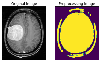
2.对图片进行阙值化处理和腐蚀处理,最后膨胀化,消除无用的噪声影响,这样使我们能更好的找到啊边界。处理后得到以下结果
3.在阙值图像中通过cv2.findContours 找到轮廓,然后抓取最大的轮廓,得到各方向的极点。
4.通过四个方向的极端点,裁剪图像,最终返回新的图像。
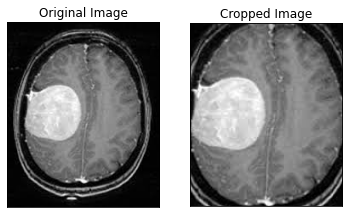
最后我们对一张图片使用裁剪功能测试功能
ex_img = cv2.imread('yes/Y1.jpg')
ex_new_img = crop_brain_contour(ex_img, True)
最终得到以下效果:
2)裁剪/waterT1C/文件夹下的png文件
题目条件:
除去图像黑边,保留脑部图像; 输入是8位png图像,输出也要求是8位png; 不要进行缩放; 一次将一个文件夹下的所有png全部裁剪完。
这里我还是参考Mohamed Ali Habib的代码进行修改。
首先查看其中一张图片的原始信息,以保证最后图像输出要求
30-T4N2, 24_pre_waterT1C.nii-0010.png: PNG image data, 512 x 512, 8-bit grayscale, non-interlaced
导入相关模块
import cv2
import imutils
import numpy as np
import matplotlib.pyplot as plt
import time
from os import listdir,makedirs

%matplotlib inline
定义裁剪函数
def crop_brain_contour(image):

    # Convert the image to grayscale, and blur it slightly
    gray = cv2.cvtColor(image, cv2.COLOR_BGR2GRAY)
    gray = cv2.GaussianBlur(gray, (5, 5), 0)

    # Threshold the image, then perform a series of erosions +
    # dilations to remove any small regions of noise
    thresh = cv2.threshold(gray, 45, 255, cv2.THRESH_BINARY)[1]
    thresh = cv2.erode(thresh, None, iterations=2)
    thresh = cv2.dilate(thresh, None, iterations=2)

    # Find contours in thresholded image, then grab the largest one
    cnts = cv2.findContours(thresh.copy(), cv2.RETR_EXTERNAL, cv2.CHAIN_APPROX_SIMPLE)
    cnts = imutils.grab_contours(cnts)
    c = max(cnts, key=cv2.contourArea)


    # Find the extreme points
    extLeft = tuple(c[c[:, :, 0].argmin()][0])
    extRight = tuple(c[c[:, :, 0].argmax()][0])
    extTop = tuple(c[c[:, :, 1].argmin()][0])
    extBot = tuple(c[c[:, :, 1].argmax()][0])

    # crop new image out of the original image using the four extreme points (left, right, top, bottom)
    new_image = image[extTop[1]:extBot[1], extLeft[0]:extRight[0]]

    return new_image
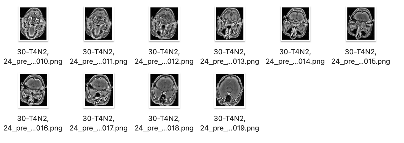
接下来对一个文件夹中的图片进行批量化处理,将其保存在waterT1CProcessed 文件夹中
makedirs('waterT1CProcessed')
for img_dir in listdir('waterT1C/'):
    ex_new_img = crop_brain_contour(cv2.imread('waterT1C/'+img_dir), True)
    cv2.imwrite('waterT1CProcessed/'+img_dir, ex_new_img)
其中一张图片的裁剪效果如下
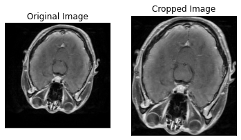
输出图片下载地址https://cdn.jsdelivr.net/gh/loyio/oss@main/Files/waterT1CProcessed.zip
然后我们查看裁剪后的图片详细信息
30-T4N2, 24_pre_waterT1C.nii-0010.png: PNG image data, 352 x 426, 8-bit/color RGB, non-interlaced
符合输出8位png的要求